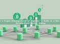
A bonding curve is a smart contract that automatically prices and creates liquidity for a token using a mathematical formula. It completely flips the traditional trading model on its head — instead of needing a buyer and a seller to match orders, you trade directly against the smart contract. Here’s the core idea: a token’s price is dynamically determined by a preset formula (like y = x²) and the current token supply. Simply put, when someone buys, the supply goes up and the price automatically rises. When someone sells, the supply goes down and the price automatically drops. This mechanism enables instant, permissionless trading, automated market making, and early price discovery. It’s widely used for community token launches, NFT fractionalization, and fundraising for DAOs (Decentralized Autonomous Organizations).
1. When Trading Doesn’t Need a Counterparty
Imagine walking up to a vending machine to buy a soda. The price is set by the machine. You put your money in, and it dispenses the drink. The whole transaction happens without haggling with another person, and you never have to worry about whether the machine is "out of stock" — as long as it’s loaded, the trade happens instantly.
In the crypto world, a bonding curve is like a supercharged version of that vending machine. Except, instead of selling physical goods, it creates and trades brand-new digital assets. By using a clever mathematical formula baked into a smart contract, it builds a 24/7 market that needs no counterparties, where the price is driven entirely by an algorithm.
This is one of the most innovative and fascinating inventions in decentralized finance (DeFi). It allows a project to go from nothing — zero liquidity, zero traders — to having a fully liquid, global market in an instant. Let’s pull back the curtain and see how it all works.
2. A Deep Dive into How Bonding Curves Work
2.1 The Core Analogy: The Magic Vending Machine
Let’s expand on that vending machine analogy:
-
A Traditional Exchange (Order Book Model): Think of this as a flea market. You want to buy a vintage vase. You have to find someone willing to sell it, negotiate a price, and then make the trade. If no one’s selling, you’re out of luck. If you can’t agree on a price, the deal dies. These are the classic problems of poor liquidity and slippage.
-
The Bonding Curve Model: This is like a "magic" vending machine. It holds a pool of tokens and a pool of reserve funds (usually a base asset like ETH or USDC). Want to buy a token? You just feed money into the machine. Following a publicly known formula, it "mints" brand-new tokens and hands them to you. Want to sell? You feed the tokens back into the machine. It "burns" (destroys) them and, following the same formula, spits out the appropriate amount of reserve funds back to you.
This is the revolutionary part: you are always trading against a program (a smart contract), never another person. The contract acts as your ultimate, always-available counterparty, providing what feels like infinite liquidity.
2.2 The Mathematical Core: How Is the Price "Calculated"?
A bonding curve is essentially a functional relationship between a token's "price" (P) and its "supply" (S) . The two most common types are:
-
Linear Curve:
P = m * S + b -
How it behaves: Each new token minted increases the price by a constant amount.
-
Example: Let’s say the formula is
P = 1 * S. The 1st token costs $1, the 2nd costs $2... the 10th token costs $10. Your cost to buy the 10th token is the price at that moment, but the total cost to buy all 10 is the sum of all those individual prices. -
Exponential Curve:
P = a * S² + b -
How it behaves: The price creeps up slowly at first, then absolutely skyrockets later on. This creates massive early-adopter incentives.
-
Example: Imagine the formula is
P = S². The 1st token is $1, the 2nd is $4, the 3rd is $9... the 10th is a whopping $100.
Key Insight: The total cost to buy a chunk of tokens isn't just price * quantity. Instead, it’s the integral (the area) under the curve from the starting supply point to the ending supply point. The smart contract uses calculus to figure out the exact amount you owe or will receive.
2.3 The Lifecycle of a Trade
Let’s walk through an example using a linear bonding curve with the formula P = 0.01 * S:
-
Deployment: A developer sets up the bonding curve smart contract. At this point, the supply
S=0and priceP=0. -
First Buyer (Alice) Steps In: She wants to buy 10 tokens.
-
The contract calculates the area under the curve to mint tokens #1 through #10.
-
A rough calculation: token 1 is $0.01, token 2 is $0.02... token 10 is $0.10. The total cost is roughly `(0.01 + 0.10) * 10 / 2 = $0.55`.
-
Alice pays $0.55 and gets 10 tokens. Supply is now `S=10`, and the new spot price is `P=$0.10`. Her $0.55 is locked securely in the contract’s "reserve pool."
-
Second Buyer (Bob) FOMOs In: He sees the price move and also wants 10 tokens.
-
The contract now calculates the cost to mint tokens #11 through #20.
-
Starting price is $0.11, ending price is $0.20. Total cost: roughly
(0.11 + 0.20) * 10 / 2 = $1.55. -
Bob pays $1.55. Supply is now `S=20`, price is `P=$0.20`.
-
Alice Takes Profit: She decides to sell her 10 tokens.
-
The contract calculates the refund for burning the last 10 tokens (tokens #20 down to #11).
-
This refund amount is identical to what Bob paid to buy them: $1.55.
-
Alice receives $1.55, netting a cool $1.00 profit. Her tokens are burned, supply drops back to
S=10, and the price falls back toP=$0.10.
A perfect, closed-loop system! No order books, no market makers, just math and code enforcing ironclad rules. The funds in the reserve pool are always mathematically guaranteed to cover the buyback of every single token in circulation.
3. Data Comparison: Bonding Curve vs. Order Book Model
Here’s a side-by-side look to make the advantages and trade-offs crystal clear.
| Feature | Bonding Curve | Traditional Order Book |
|---|---|---|
| Counterparty | The smart contract itself. Always present, provides instant liquidity. | Other market participants. A buyer must be matched with a seller. |
| Pricing Mechanism | Algorithm-driven. Price is auto-calculated by supply based on a preset formula. | Supply-and-demand-driven. Price is discovered through bids and asks. |
| Liquidity Needs | Liquidity is created from day one. No critical mass of users or capital needed. | Has a cold-start problem. A new asset has terrible liquidity and is hard to trade. |
| Price Slippage | Predictable slippage. Determined by the curve’s shape; completely transparent. | Unpredictable slippage. Depends on order book depth; large orders move the market hard. |
| Barrier to Entry | Very low. Anyone can buy or sell anytime without waiting for a match. | Higher. Users must understand limit vs. market orders and may wait for fills. |
| Typical Use Cases | Community token launches, continuous fundraising, NFT fractionalization, in-game assets. | Blue-chip crypto, mature project tokens, stocks, futures, mainstream finance. |
| Key Advantage | Instant liquidity, automated market making, early price discovery, built-in incentives. | More granular price discovery, supports complex order types (stop-loss, limit). |
| Key Risk | Smart contract bugs, poorly designed curve models leading to crashes or pump-and-dumps. | Market manipulation, liquidity drying up, counterparty risk. |
4. Q&A Section
Q1: What exactly is the "reserve pool" in a bonding curve, and is it safe?
A: The reserve pool is where the base asset (like ETH) that buyers pay gets stored. It’s held in escrow by the smart contract. Its sole job is to act as collateral to buy back tokens. As long as the smart contract code has no vulnerabilities, the funds are safe and can’t be rugged or stolen. The math ensures the value in the pool perfectly backs the market cap of all outstanding tokens.
Q2: What if I'm the very last person holding the token? Can I still sell?
A: Absolutely. This is one of the biggest selling points. As long as the curve’s formula is active, the smart contract is the ultimate buyer of last resort. Even if everyone else on earth has sold, you can always sell your tokens back to the contract and reclaim your fair share of the reserve pool. You can never be left holding a bag that’s completely worthless and unsellable.
Q3: What are the common types of bonding curves and where are they used?
A: There are a few key variants:
-
Single-Sided Curve: The classic model from our examples. Used to launch a single project token against a reserve asset.
-
Buy/Sell Split Curves (Double Curve): The buy and sell functions are different. Typically, the selling price is slightly lower than the buying price (creating a spread). This difference can flow into a project treasury for ongoing development.
-
Multi-Token Curves: This is exactly what Uniswap’s
x * y = kconstant product formula is. It links two assets to create an automated market maker (AMM). -
Applications: Community currencies, prediction markets, creator tokens/content monetization, and NFT fractionalization/buyouts.
Q4: What are the risks and downsides of bonding curves?
A: The main risks are: ① Smart contract vulnerabilities — a hack is the biggest existential threat. ② Poorly designed curve models — a curve that’s too steep can become a speculative bubble that collapses violently. ③ Lack of advanced trading features — you can’t place a limit order. ④ Information asymmetry — insiders and early adopters can have an unfair advantage over latecomers. ⑤ Reserve asset risk — if the reserve asset (e.g., ETH) itself crashes in value, it drags the token price down with it.
Q5: Why do early buyers make so much profit? Isn't that unfair?
A: Think of this as a feature, not a bug. It’s a fundamental risk/reward trade-off. Early participants are taking the biggest risks—unproven code, potential for total failure, zero initial liquidity. In return, they get the lowest entry price. This mechanism brilliantly incentivizes the early believers and evangelists who bootstrap the project. Whether that’s "fair" ultimately depends on community consensus and full transparency from the project.
Q6: How is a bonding curve related to Uniswap and other AMMs?
A: You can think of Uniswap’s constant product market maker model (x * y = k) as a specific, sophisticated type of bonding curve. It’s a two-way curve that connects two assets and ensures their product remains constant. Generally, when people say "bonding curve," they’re more narrowly referring to the single-asset issuance model (depositing one asset to mint a new one).
Q7: Can anyone just create a bonding curve and launch their own token?
A: Yes, and it’s dead simple now. Many platforms (like Gitcoin’s Aqueduct, Rug.fyi, Zora’s auction tools) offer one-click creation. You don’t need any coding skills. You just set your parameters (initial price, slope, token supply cap, etc.), and you can deploy your own bonding curve token in minutes. It has massively lowered the barrier to entry for tokenizing a community or project.
5. Conclusion
The bonding curve is a beautiful fusion of cryptoeconomic theory and decentralized governance ideals. It transforms a cold, hard mathematical formula into a vibrant, self-organizing market.
Here’s what it brings to the table:
-
Liquidity from Ground Zero: It completely solves the cold-start problem that plagues new projects.
-
Algorithmic Fairness: Prices aren’t set by backroom deals or manipulative whales, but by transparent, auditable code.
-
Frictionless, Continuous Trading: A 24/7/365 market where trades execute instantly.
-
Built-in Long-Term Incentives: It rewards early believers and creates a self-propagating community network.
It’s not a perfect solution — challenges with model design and smart contract security are real — but it undeniably offers a radically new paradigm for creating, distributing, and discovering the value of digital assets. Understanding the bonding curve is like understanding a foundational building block of the decentralized world. It’s more than just a tech tool; it’s a grand experiment in assets, community, and economic models.